Machine Learning Fundamentals

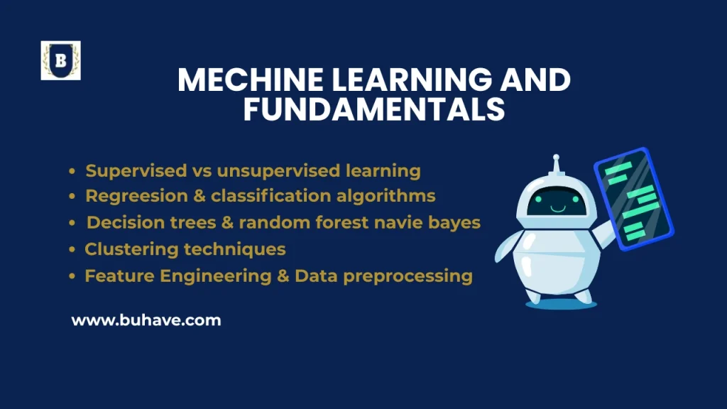
Supervised vs Unsupervised Learning

Machine Learning is broadly categorized into Supervised and Unsupervised Learning. Let’s break them down.

Supervised Learning

Definition: The model learns from labeled data (input-output pairs).

Goal: Map inputs to outputs by minimizing error.

Example: Given house features (size, location, etc.), predict price.

Types of Supervised Learning

1- Regression: Predict continuous values.

• Example: Predicting temperature based on past data.
• Algorithms: Linear Regression, Decision Trees, Neural Networks.

2- Classification: Predict discrete categories.

• Example: Spam detection (Spam/Not Spam).
• Algorithms: Logistic Regression, SVM, Random Forest, Neural Networks

Supervised Learning in Python

from sklearn. linear  _ model import Linear Regression
import numpy as np

# Training data (features and labels)
X = np. array([[1], [2], [3], [4], [5]]) # Input: Hours studied
y = np. array([50, 60, 70, 80, 90]) # Output: Exam scores

# Train model
model = Linear Regression()
model. fit(X, y)

# Predict for 6 hours of study
prediction = model. predict([[6]])
print(“Predicted Score:”, prediction[0])

Unsupervised Learning

Definition: The model learns from unlabeled data (no explicit outputs).

Algorithm: Find hidden patterns or groupings in data.

Example: Grouping customers based on purchase behavior.

Types of Unsupervised Learning

1- Clustering: Group similar data points.

• Example. : Customer segmentation in marketing.
• Algorithms: K-Means, DBSCAN, Hierarchical Clustering.

2- Dimensionality Reduction: Reduce feature space.

• Example : Compressing image data while retaining key features.
• Algorithms: PCA, t-SNE, Autoencoders.

Unsupervised Learning in Python

from sklearn. cluster import KMeans

# Sample data (age, income)
X = np. array([[25, 50000], [30, 60000], [35, 70000], [40, 80000], [45, 90000]])

# Train K-Means model
kmeans = KMeans (n_clusters=2, random_state=42)
kmeans. fit(X)

# Predict cluster for a new person
prediction = kmeans. predict([[32, 62000]])
print(“Cluster:”, prediction[0])

Key Differences: Supervised vs Unsupervised Learning

Feature	Supervised Learning	Unsupervised Learning
Labels	Labeled data	No labels
Goal	Predict outcomes	Find patterns
Example Task	Spam detection, Price prediction	Customer segmentation
Algorithms	Linear Regression, SVM, Neural Networks	K-Means, PCA, Autoencoders

Next Steps:

• Want to explore semi-supervised or reinforcement learning?
• Need hands-on practice with a dataset?

Regression & Classification Algorithms in Machine Learning

In Supervised Learning, we deal with Regression (continuous output) and Classification (discrete output). Let’s explore both!

1. Regression Algorithms (Predicting Continuous Values)

Definition: Regression predicts a continuous numerical value (e.g., house prices, temperature, stock

Example: Predicting a person’s salary based on experience.

Common Regression Algorithms:

Algorithm	Description
Linear Regression	Models a linear relationship between input and output.
Polynomial Regression	Extends linear regression with polynomial features.
Decision Trees (CART)	Splits data into decision-based segments for prediction.
Random Forest	Uses multiple decision trees and averages results.
Support Vector Regression (SVR)	Finds a hyperplane in higher dimensions to predict values.
Neural Networks (Deep Learning)	Uses layers of neurons to learn complex relationships.

Linear Regression in Python

from sklearn. linear _ model import Linear Regression
import numpy as np

# Training data (Experience in years & Salary)
X = np. array([[1], [2], [3], [4], [5]]) # Years of experience
y = np. array([30000, 40000, 50000, 60000, 70000]) # Salary

# Train model
model = Linear Regression()
model. fit(X, y)

# Predict salary for 6 years of experience
prediction = model. predict([[6]])
print(“Predicted Salary:”, prediction[0])

2. Classification Algorithms (Predicting Categories)

Definition: Classification predicts a categorical label (e.g., spam/not spam, fraud detection, disease

Example: Classifying whether an email is spam or not spam.

Common Classification Algorithms:

Algorithm	Description
Logistic Regression	A statistical model for binary classification (e.g., Yes/No).
K-Nearest Neighbors (KNN)	Classifies based on the majority of k-nearest neighbors.
Decision Trees (CART)	Splits data into decision rules for classification.
Random Forest	Uses multiple decision trees and majority voting.
Support Vector Machine (SVM)	Finds the best hyperplane to separate classes.
Naïve Bayes	Based on Bayes’ Theorem, used for text classification.
Neural Networks (Deep Learning)	Uses multiple layers to learn complex patterns.

Logistic Regression in Python

from sklearn.linear_model import LogisticRegression

# Training data (Hours studied & Pass/Fail labels)
X = np.array([[1], [2], [3], [4], [5]]) # Hours studied
y = np.array([0, 0, 0, 1, 1]) # 0 = Fail, 1 = Pass

# Train model
model = LogisticRegression()
model.fit(X, y)

# Predict pass/fail for 3.5 hours of study
prediction = model.predict([[3.5]])
print(“Predicted Outcome (0=Fail, 1=Pass):”, prediction[0])

Key Differences: Regression vs Classification

Feature	Regression	Classification
Output Type	Continuous values (e.g., price)	Discrete categories (e.g., Yes/No)
Example Task	House price prediction	Spam detection
Common Algorithms	Linear Regression, SVR, Neural Networks	Logistic Regression, SVM, Decision Trees
Evaluation Metrics	RMSE, MAE, R² score	Accuracy, Precision, Recall, F1-score

Next Steps:

• Want to explore deep learning models for regression/classification?
• Need help choosing the best algorithm for your dataset?

Decision Trees, Random Forest, Naïve Bayes

1. Decision Trees (CART – Classification and Regression Trees)

• A tree-based model that splits data into smaller subsets based on feature conditions.
• A series of “Yes/No” questions leading to a final prediction.
• Both classification (e.g., spam detection) and regression (e.g., house price prediction

Example:

• If weather = sunny → play outside
• If weather = rainy → stay inside

Pros & Cons:

• Easy to interpret & visualize
• Works well on structured/tabular data
• No need for feature scaling
• Prone to overfitting (high variance)
• Unstable if small changes in data occur

Decision Tree in Python

from sklearn. tree import Decision Tree Classifier

# Sample data (features: Weather, Temperature) and labels (Play: Yes/No)
X = [[0, 30], [1, 20], [0, 25], [1, 15], [0, 35]] # (0=Sunny, 1=Rainy)
y = [1, 0, 1, 0, 1] # (1=Play, 0=Don’t play)

# Train model
model = Decision Tree Classifier()
model. fit(X, y)

# Predict for (Rainy, 28°C)
prediction = model. predict([[1, 28]])
print(“Play outside?”, “Yes” if prediction[0] == 1 else “No”)

2. Random Forest (Ensemble Learning)

• A collection of multiple Decision Trees combined to improve accuracy and reduce overfitting.
• Builds multiple trees and averages predictions (regression) or takes majority vote (classification).
• Fraud detection, medical diagnosis, stock market prediction, etc.

Pros & Cons:

• More accurate & stable than a single decision tree
• Handles missing values & categorical features well
• Reduces overfitting
• Slower training time for large datasets
• Harder to interpret

Random Forest in Python

from sklearn. ensemble import Random Forest Classifier

# Sample data (same as Decision Tree example)
X = [[0, 30], [1, 20], [0, 25], [1, 15], [0, 35]]
y = [1, 0, 1, 0, 1]

# Train model with multiple trees
model = RandomForestClassifier(n_estimators=100, random_state=42)
model.fit(X, y)

# Predict for (Rainy, 28°C)
prediction = model.predict([[1, 28]])
print(“Play outside?”, “Yes” if prediction[0] == 1 else “No”)

3. Naive Bayes (Probabilistic Classifier)

• A classification algorithm based on Bayes’ Theorem with an assumption that features are independent.
• Uses probability to classify data points.
• Spam filtering, sentiment analysis, medical diagnosis, etc.

Types of Naive Bayes:

• Gaussian Naive Bayes: Assumes normal distribution (good for continuous data).
• Multinomial Naive Bayes: Used for text classification (e.g., spam detection).
• Bernoulli Naive Bayes: Works for binary features (e.g., word presence/absence in a document).

Pros & Cons:

• Fast and works well with small datasets
• Handles high-dimensional data well (e.g., text data)
• Works well with probabilistic models
• Assumes independence between features (not always true)
• Can be biased if dataset doesn’t follow assumptions

Naive Bayes in Python

from sklearn. naive_bayes import Gaussian NB

# Sample data (features: [Height, Weight], label: Male(1)/Female(0))
X = [[170, 65], [180, 80], [160, 55], [175, 75], [165, 60]]
y = [1, 1, 0, 1, 0] # 1 = Male, 0 = Female

# Train model
model = GaussianNB()
model.fit(X, y)

# Predict for a person with (Height=172cm, Weight=68kg)
prediction = model. predict([[172, 68]])
print(“Predicted Gender:”, “Male” if prediction[0] == 1 else “Female”)

Decision Tree vs Random Forest vs Naive Bayes

Feature	Decision Tree	Random Forest	Naive Bayes
Type	Tree-based Model	Ensemble Learning	Probabilistic Model
Overfitting	High risk	Low risk	Low risk
Speed	Fast	Slower than DT	Fastest
Interpretability	Easy to understand	Harder than DT	Less intuitive
Best For	Structured data	Complex datasets	Text & probabilistic data

Next Steps:

• Want to apply these models to real-world datasets?
• Need help tuning hyperparameters

Clustering Techniques: K-Means, DBSCAN

Clustering is an Unsupervised Learning technique used to group similar data points together. Two of the most popular clustering algorithms are K-Means and DBSCAN. Let’s dive in!

1. K-Means Clustering

K-Means partitions data into K clusters, where each point belongs to the nearest cluster center (centroid).

How It Works:

• Choose K (number of clusters).
• Initialize K centroids randomly.
• Assign each point to the nearest centroid.
• Update centroids as the mean of assigned points.
• Repeat steps 3-4 until centroids don’t change (convergence).

Used For:

• Customer segmentation
• Image compression
• Anomaly detection

Pros & Cons of K-Means:

• Fast & scalable for large datasets
• Works well with well-separated clusters
• Must manually choose K (not always obvious)
• Struggles with non-spherical clusters & outliers

K-Means in Python:

from sklearn. cluster import KMeans
import numpy as np

# Sample dataset (2D points)
X = np.array([[1, 2], [1, 4], [1, 0],
[10, 2], [10, 4], [10, 0]])

# Train K-Means model with K=2 clusters
kmeans = KMeans(n_clusters=2, random_state=42)
kmeans.fit(X)

# Predict cluster for a new point
prediction = kmeans.predict([[5, 3]])
print(“Cluster:”, prediction[0])

2. DBSCAN (Density-Based Clustering)

DBSCAN (Density-Based Spatial Clustering of Applications with Noise) groups points that are densely packed together and labels sparse points as outliers.

How It Works:

• Define ε (epsilon) (radius) and MinPts (minimum points to form a cluster).
• Pick a random point and check its ε-neighborhood.
• If it has MinPts neighbors, it’s a core point → forms a cluster.
• Expand the cluster by adding nearby points.
• Mark isolated points as noise (outliers).

Used For:

• Anomaly detection (fraud detection)
• Geospatial data clustering (earthquake zones)
• Non-spherical data (e.g., moon-shaped clusters)

Pros & Cons of DBSCAN:

• No need to specify K (auto-detects clusters)
• Handles outliers well (labels them as noise)
• Works well for arbitrarily shaped clusters
• Not scalable for large datasets
• Sensitive to ε & MinPts values

DBSCAN in Python:

from sklearn. cluster import DBSCAN

# Sample dataset (2D points)
X = np. array([[1, 2], [2, 3], [2, 2],
[8, 7], [8, 8], [25, 80]])

# Train DBSCAN model
dbscan = DBSCAN(eps=2, min_samples=2)
dbscan.fit(X)

# Cluster labels (-1 means noise/outlier)
print(“Cluster Labels:”, dbscan.labels_)

K-Means vs. DBSCAN:

table {
width: 100%;
border-collapse: collapse;
}
th, td {
border: 1px solid #ddd;
padding: 8px;
text-align: left;
}
th {
background-color: #f2f2f2;
}

K-Means vs DBSCAN

Feature	K-Means	DBSCAN
Cluster Shape	Works well for spherical clusters	Works for arbitrary shapes
Handling Outliers	Sensitive to outliers	Detects outliers
Number of Clusters	Must predefine K	Automatically detects
Scalability	Fast for large datasets	Slower for large datasets
Best For	Customer segmentation, image compression	Anomaly detection, geospatial clustering

Next Steps:

• Want to visualize clustering results?
• Need help choosing parameters like K (for K-Means) or eps (for DBSCAN)?

Feature Engineering & Data Preprocessing

Before training a machine learning model, raw data needs to be cleaned, transformed, and optimized. This process is called Feature Engineering & Data Preprocessing.

1. Data Preprocessing

Data preprocessing is about cleaning and preparing data for modeling. Here are 3 steps in Data Preprocessing:
1. Handling Missing Values

• Remove rows/columns with too many missing values
• Fill missing values using mean, median, mode, or imputation techniques

from sklearn.impute import SimpleImputer
import numpy as np

# Sample dataset with missing values
X = np.array([[1, 2], [np.nan, 3], [7, 6]])

# Fill missing values with column mean
imputer = SimpleImputer(strategy=’mean’)
X_filled = imputer.fit_transform(X)
print(X_filled)

2. Handling Categorical Data (Encoding)

• One-Hot Encoding for categorical variables (e.g., “Red”, “Blue”, “Green”)
• Label Encoding for ordinal categories (e.g., “Low”, “Medium”, “High”)

from sklearn. preprocessing import One Hot Encoder

# Sample categorical data
categories = np.array([[“Red”], [“Blue”], [“Green”]])

# One-hot encoding
encoder = OneHotEncoder(sparse=False)
encoded_categories = encoder.fit_transform(categories)
print(encoded_categories)

3. Feature Scaling (Normalization & Standardization)

• Min-Max Scaling: Scales values between 0 and 1
• Standardization (Z-score normalization): Transforms data to have zero mean and unit variance

from sklearn. preprocessing import Standard Scaler, Min Max Scaler

# Sample data
X = np.array([[1, 2], [3, 4], [5, 6]])

# Min-Max Scaling
scaler = Min Max Scaler()
X_scaled = scaler.fit_transform(X)
print(X_scaled)

# Standardization
scaler = Standard Scaler()
X_standardized = scaler. fit_transform(X)
print(X_standardized)

2. Feature Engineering

Feature Engineering is the process of creating new features or modifying existing ones to improve model performance.

Feature Engineering Techniques:

• Feature Creation: Combine existing features to create new meaningful ones (e.g., BMI = weight / height^2).
• Feature Selection: Remove irrelevant or redundant features.
• Polynomial Features: Create interaction terms (e.g., x1 * x2).
• Dimensionality Reduction: Use PCA to reduce features while retaining important information.

from sklearn. decomposition import PCA

# Sample dataset with 3 features
X = np.array([[2, 3, 4], [5, 6, 7], [8, 9, 10]])

# Reduce to 2 principal components
pca = PCA(n_components=2)
X_reduced = pca.fit_transform(X)
print(X_reduced)

Next Steps:

• Want help cleaning a dataset?
• Need guidance on feature selection techniques?

Hands-on Practice – Machine Learning:

1- Train a Linear Regression Model using scikit-learn

Let’s train a Linear Regression model using Scikit-learn on a sample dataset.

Step 1: Import Libraries:

import numpy as np
import matplotlib. pyplot as plt
from sklearn. model _ selection import train _ test _ split
from sklearn. linear _ model import Linear Regression
from sklearn. metrics import mean _ squared _ error

Step 2: Generate Sample Data:
We’ll create a simple linear relationship.

y = 3x + 5 + noise

# Generate synthetic dataset
np. random. seed(42)
X = 2 * np. random. rand(100, 1) # Features (100 samples)
y = 3 * X + 5 + np. random. randn(100, 1) # Target variable with noise

Step 3: Train-Test Split:
We split our dataset into 80% training and 20% testing.

X _ train, X _ test, y _ train, y _ test = train _ test _ split(X, y, test _ size=0.2, random _ state=42)

Step 4: Train the Linear Regression Model:
We fit the model on the training data.

# Train Linear Regression model
model = LinearRegression()
model.fit(X_train, y_train)

Step 5: Model Evaluation:
Let’s check the model’s coefficients and performance.

# Get model parameters
print(f”Intercept: {model. intercept_[0]}”)
print(f”Coefficient: {model. coef_[0][0]}”)

# Make predictions
y _ pred = model. predict(X _ test)

# Calculate Mean Squared Error (MSE)
mse = mean _ squared _ error(y _ test, y _ pred)
print(f”Mean Squared Error: {mse:.2f}”)

Step 6: Visualization:
Let’s plot the actual data vs. predicted regression line.

plt.scatter(X_test, y_test, color=”blue”, label=”Actual Data”)
plt.plot(X_test, y_pred, color=”red”, linewidth=2, label=”Regression Line”)
plt.xlabel(“X”)
plt.ylabel(“y”)
plt.legend()
plt.title(“Linear Regression Model”)
plt.show()

Output & Interpretation:

• The intercept (~5) and coefficient (~3) match our original equation y = 3x + 5.
• The red line represents the learned relationship between X & y.
• Lower MSE means a better fit.

2- Implement K-Means Clustering on real-world datasets

Let’s apply K-Means Clustering to a real-world dataset using Scikit-learn. We’ll use the Iris dataset, a popular dataset in machine learning.

Step 1: Import Libraries:

import numpy as np
import pandas as pd
import matplotlib. pyplot as plt
import seaborn as sns
from sklearn. cluster import KMeans
from sklearn. datasets import load_iris
from sklearn. preprocessing import Standard Scaler

Step 2: Load the Iris Dataset:

The Iris dataset contains 150 samples of iris flowers, categorized into 3 species (Setosa, Versicolor, Virginica).

Each sample has 4 features:

1. Sepal Length
2. Sepal Width
3. Petal Length
4. Petal Width

Example:

# Load Iris dataset
iris = load_iris()
df = pd. Data Frame(iris. data, columns=iris.feature _ names)
df. head()

Step 3: Data Preprocessing (Feature Scaling):
Since K-Means is distance-based, it’s important to normalize the features.

scaler = StandardScaler()
df _ scaled = scaler.fit _ transform(df)

Step 4: Determine the Optimal Number of Clusters (Elbow Method):
The Elbow Method helps find the best K by plotting inertia (sum of squared distances).

inertia = []
K _ range = range(1, 11)

for k in K _ range:
kmeans = KMeans(n_clusters=k, random_state=42)
kmeans. fit(df _ scaled)
inertia. append(kmeans.inertia_)

# Plot the Elbow Method
plt. figure(figsize=(8,5))
plt. plot(K _ range, inertia, marker=’o’, linestyle=’–‘)
plt. xlabel(“Number of Clusters (K)”)
plt. ylabel(“Inertia (Sum of Squared Distances)”)
plt. title(“Elbow Method for Optimal K”)
plt. show()

Interpretation: Look for the “elbow point” where inertia starts decreasing at a slower rate. This is the optimal K.

Step 5: Apply K-Means Clustering:
Let’s choose K=3 (from the elbow method) and apply K-Means.

# Train K-Means model
kmeans = KMeans (n _ clusters=3, random _ state=42)
df[“Cluster”] = kmeans. fit _ predict(df _ scaled)

# Check cluster assignment
df.head()

Step 6: Visualizing Clusters (Using First Two Features):
Since the dataset has 4 dimensions, we’ll use only Sepal Length & Sepal Width for visualization.

plt.figure(figsize=(8,6))
sns. scatterplot(x=df[iris. feature _ names[0]], y=df[iris. feature _ names[1]], hue=df[“Cluster”], palette=”viridis”)
plt.scatter(kmeans. cluster _ centers_[:,0], kmeans. cluster _ centers_[:,1], color=’red’, marker=’X’, s=200, label=”Centroids”)
plt.xlabel(“Sepal Length”)
plt.ylabel(“Sepal Width”)
plt.title(“K-Means Clustering on Iris Dataset”)
plt.legend()
plt.show()

Key Takeaways

• K-Means successfully groups the dataset into 3 clusters (matching the 3 iris species).
• The Elbow Method helps find the best K.
• Feature scaling is essential for accurate clustering.

Write for us in Education and submit guest posts for publishing at admin@buhave.com